In this course, we will begin with a basic understanding of perception and the functionalities of perception algorithms. We will provide a high-level overview of the typical mobile robotic perception to serve as a practical reference for the topics covered in the later part of the course. Then we will cover the topic of localization and how they are used in a typical mobile robotic system or an autonomous vehicle.

1. Perception: Indoor and Outdoor

2. Mapping and Localization

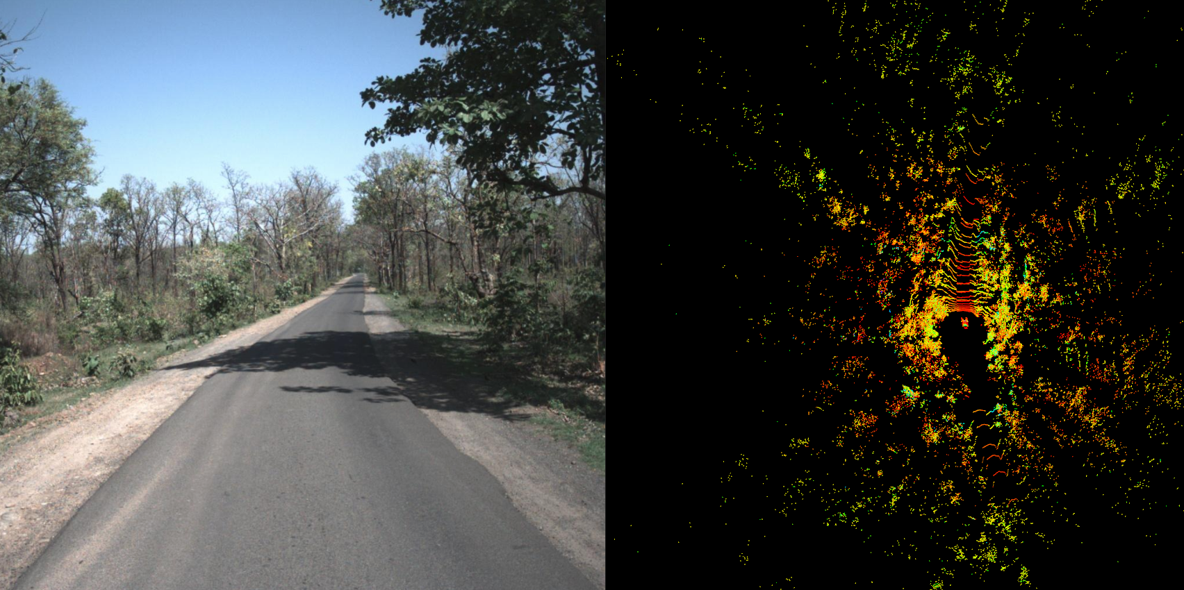
In Autonomous Driving sensors such as Cameras, LiDARs, and RADARs play critical roles in enabling self-driving vehicles to perceive their environment and make informed decisions. Let's delve into their significance and then shift our focus to the intricate world of computer vision, emphasizing the nuances of camera sensors.

1. Sensors: LiDARs and Cameras, RADAR

2. Images and Image Channels

    a. Image Channels

    b. Coordinate Conventions

3. Color Spaces

    a. Image Color Spaces (RGB, Gray Scale, HSV etc...)

This segment of the course will delve into the comprehensive exploration of Noise Models, a pivotal area of research and development in computer vision and image processing. We will thoroughly investigate three fundamental noise models: Uniform Noise, Gaussian Noise, and Impulse Noise. Understanding these models is vital for developing advanced image denoising techniques, enhancing the robustness of computer vision algorithms, and improving the reliability of autonomous systems in noisy real-world environments. Ongoing research in this domain seeks to create innovative noise reduction methodologies, leveraging cutting-edge deep learning and statistical approaches, to push the boundaries of image quality and perception in autonomous driving and beyond.

1. Uniform Noise

2. Gaussian Noise

3. Substitutive Noise Models

4. Impulse Noise

5. Salt and Pepper Noise

We will begin the topic of Image Enhancement in this part of the course, and cover the fundamentals which will be helpful for understanding further lectures in the coming parts. We will briefly present the Spatial Domain and Frequency Domain processing methods, introduce filters, and provide a motivation for the contrast enhancement in images. We will end this part of the course with the image histograms (including normalized histogram), for both the color and gray scale images. The rest of the topics under image enhancement will be covered in the part-3 of the course.

1. Spatial vs Frequency Domain

2. Spatial Domain Processing

3. Histogram Equalization: Motivation and Algorithm

4. Adaptive Histogram Equalization

5. CLAHE

Image smoothing is a critical and ever-evolving facet of image processing and computer vision algorithms. In this course segment, we will not only introduce the fundamental concept of image smoothing but also delve into advanced techniques. We will explore correlation and convolution methods, essential for smoothing and feature extraction. Furthermore, we will provide an in-depth analysis of a diverse array of filters employed in image smoothing

1. Image Smoothing

    a. Filters

    b. Correlation vs Convolution

    c. Uniform Filter

    d. Gaussian Filter

    e. Geometric Mean Filter

In this segment of the course we'll cover morphological operations like dilation and erosion, with their fundamental set theoretic explanation. We'll also explain opening and closing operations for shape analysis and introduce morphological image smoothing for binary images, aiding various applications in computer vision.

1. Morphological Image Operations

2. Set Theory

3. Hit and Fit

4. Structuring Element

5. Morphological Dilation and Erosion

6. Set Theoretic Explanation of Dilation

7. Set Theoretic Explanation of Erosion

8. Erosion and Dilation: Duality

9. Opening, Closing

10. Morphological Image Smoothing

In this course segment, we delve into two sophisticated image smoothing algorithms renowned for their ability to preserve edges effectively. We explore the intricate mathematics behind Bilateral Filtering and Kuwahara Filtering, revealing the inner workings of these techniques. By understanding these algorithms in-depth, participants gain valuable insights into how to achieve advanced image smoothing while maintaining the essential features of the original image. This knowledge serves as a cornerstone for researchers and practitioners striving to enhance image processing techniques in fields such as medical imaging, computer vision, and beyond.

1. Bilateral Filter

2. Bilateral vs Gaussian Filter

3. Kuwahara Filter

4. Kuwahara Filter and Bilateral Filter Comparison

This course module is dedicated to the fundamental concept of edge detection in image processing, a cornerstone of computer vision and image analysis. We begin by exploring first-order edge detection methods, laying the foundation for understanding image gradients and the detection of abrupt intensity changes. Moving beyond, we introduce second-order techniques, particularly the Laplacian operator, which enhances our ability to pinpoint edges by emphasizing intensity variations. However, this module extends beyond theory. It forms the basis for comprehending the powerful Laplacian of Gaussian filter, a pivotal tool in edge detection and feature extraction. This filter not only aids in identifying edges but also serves in general feature detection, particularly for spotting objects like blobs.

1. Pixel Connectivity

2. Edge Point

3. Digital Approximation of First Order Derivative

4. First-Order Methods

    a. Sobel Operator

    b. Prewitt Operator

    c. Scharr Operator

5. Digital Approximation of 2nd Order Derivative

6. Laplacian: Features

7. Edge Detection using Laplacian Operator

8. Introduction to LoG (Laplacian of Gaussian)

9. Zero Crossing in Second Order Methods

10. Canny Edge Detection

11. Non-Maximal Suppression

12. Double Thresholding

13. Edge Tracking via Hysteresis

This course segment marks the initiation of our exploration into visual features, a crucial domain within computer vision. We begin by unraveling the essence of visual features, delving into their distinctive properties that make them standout within images. Building the foundational understanding of visual features, we introduce two key categories: corners and blobs. In doing so, we draw comparisons with edges, enabling a comprehensive grasp of what truly constitutes robust and informative features in an image. As we delve deeper, we not only establish the mathematical underpinnings of feature detection but also embark on an exploration of algorithms tailored for corner detection in images. These algorithms are the bedrock of modern computer vision applications, facilitating everything from object tracking to scene recognition

1. Visual Features

2. Corners and Edges

3. Corners: Structural Property

4. Introduction to Blobs

5. Corner Detectors

    a. Moravec Feature Detector

    b. Harris Corner Detector

    c. Harris Mathematics: Taylor Series Approximation

    d. Harris Mathematics: Computing Matrix M

    e. Harris Mathematics: Eigenvalue Analysis

    f. Harris Mathematics: Corner Score Function

    g. Shi-Tomasi: Mathematics and Algorithm

This part of the course begins with the topic of blob detection in images, and discusses the necessary background theory, which will form the foundations of understanding the typical blob detection algorithmic pipelines. The typical blob detection pipelines are based on Laplacian of Gaussian (LoG), Difference of Gaussian (DoG), or sometimes Determinant of Hessian (DoH) based. This lecture covers both the LoG and DoG operators and algorithms based on DoG and LoG operators. The determinan of Hessian (DoH) was initially not part of this course, as it is too mathematical for the Category-II course, but now it has also been incorporated in the course as an additional interesting topic, which will improve your fundamental mathematical understanding of the blob detection literation computer vision, and also will help you in the understanding of the popular SIFT algorithm. This part of the course will cover the blob detection fundamental, will teach the importance of scalable blob detectors. It will then introduce the center surround property of the blob detectors, as to why it forms a good blob detector, and then cover the LoG, and DoG algorithms for blob detection.

1. Introduction and Characteristics

2. Center Surround Filters

3. Scalable Blob Detectors

4. Scale Normalization

5. Blob Detection using LoG Operator

6. DoG Operator

7. DoG Algorithm for Blob Detection

This part of the course deeply covers the concepts of constructing scaled representations of an input image, to facilitate feature detection a varying scales. In the previous parts of the course, we emphasized the importance of blob detectors, or generic feature detectors, being able to operate at varying scales in an image. In the previous parts, we primarily constructed algorithmic pipelines where detectors were operating at varying scales. The computer vision literature provides us some of the methodologies that help us in constructing scaled versions of the images, which inherently scale the features as well in images. In this part of the course, we will thus study methods that allows construction of such representations. We will also briefly discuss how the promiment blob decectors, such as the SIFT, exploits these ideas to construct a robust blob detector. We will thus discuss, Image Pyramids and their limitations, and then how the Gaussian Pyramids overcome those limitations. We will then disucss the Gaussian Scale Space, which is significant improvement over the Gaussian Pyramid. We will then finally cover the most important concept, the Octaves, which are obtained by combining Gaussian Scale Space with either the Gaussian Pyramid or Image Pyramid. After covering the scale space and octaves discussion, this part finally ends the topic of Blob Detection by covering additional topics under Determinant of Hessian, that were initially not part of the course outline. This part covers indepth mathematics behind the DoH as blob detector, and DoH as an eliminator of false positive blob responses in image, and the score function used by the SIFT algorithm to do so.

1. Image Pyramid and Image Scale Space

2. Aliasing Effect

3. Gaussian Image Pyramid

4. Gaussian Scale Space

5. Image Octaves

6. Octaves and DoG: Blob Detection

7. Determinant of Hessian

8. DoH: Blob Detection

9. DoH: As Eliminator (SIFT)

This part of the course covers image feature descriptors. Feature descriptor are both local and global. There are many local descriptors in the literature, but the global descriptors are limited. Thus, in this part of the course, we first make a general introduction to the feature descriptors, and then discuss the characteristics of a good feature descriptor. We also cover what local and global descriptors are used for. While the number of feature descriptors is an exhaustive list, we cover some of the most common, yet prominent descriptors, so that you get an idea of what typically feature descriptors are, and can build upon the course content with further independent readings of your own. We have added one more additional topic to the course, which was initially not part of the course outline, the GIST image descriptor, which uses a bank of Gabor Filters. Gabor Filters was initially not part of this course, as it reuqires computations in the frequency domain. In this part, we will cover extensively the BRIEF image descriptor, and then the later parts of the course will cover HoG, and Gabor Filter Banks, and then the GIST image descriptor. GIST is a global image descriptor.

1. Characteristics of Good Descriptors

2. BRIEF Descriptor

    a. Mathematics

    b. Smoothing

    c. Sampling Methods

    d. Pseudocode

3. ORB

    a. Introduction

    b. Orientation and Intensity Centroid

4. Rotated BRIEF: rBRIEF

5. HoG

    a. Algorithm

    b. Histogram Computation and Block Normalization

    c. Pseudocode

This part of the course covers another additional added topic to the course, which was not part of the course outline earlier, i.e. the Gabor Filter, Gabor Filter Banks, and the GIST Image Descriptor. In the previous sections we covered feature descriptors, that were local, i.e., they were designed with a specific purpose of describing a small patch around a feature point in an image. In this lecture we will briefly cover what global descriptors are, and also discuss the GIST Image descriptor, and along with it cover the Gabor filter, Gabor Filters bank, and how we can use Gabor filters to also compute the local texture orientation in images.

1. Global Descriptors

2. GIST

3. Gabor Filter

4. Gabor Transform Function and Gabor Filters Bank

5. GIST Descriptor Algorithm

This course segment commences with a formal introduction, setting the stage for a comprehensive exploration of the K-Means clustering algorithm. Furthermore, it delves into Kernel Density Estimation (KDE), a method frequently encountered in machine learning and statistics literature. KDE plays a pivotal role in estimating the probability density function of a dataset, shedding light on the underlying, often concealed, data generation process. Crucially, the gradient of the estimated density function serves as a powerful tool to unveil modes within the true density function. These modes pinpoint regions of high data density, crucial for clustering. The non-parametric Mean-Shift clustering algorithm is the key to identifying and associating data points with these modes, ultimately forming clustered datasets. To grasp the intricacies of Mean-Shift, a profound understanding of the foundational theory is imperative. This course module delves into this background theory, serving as the bedrock for comprehending Mean-Shift's applications in computer vision and a multitude of other fields.

1. Clustering and Image Segmentation

2. K-Means Clustering

    a. Loss Function

    b. Algorithm

    c. Pseudocode

    d. Limitations

3. K-Means++

4. Non-Parametric Clustering and Kernel Density Estimation

5. Kernel Functions in KDE

6. Generalized Kernel Density Estimator Function

7. Density Gradient Estimation

8. Mean Shift Clustering

    a. Naive Mean Shift Clustering Algorithm

    b. Mean-Shift Image Smoothing with Edge Preservation

    c. Mean-Shift Image Segmentation